Sampling Without a Statistics Degree: How to Choose the Right Sample Size for Your Field Survey
A practical guide for MEL practitioners who need rigorous enough, not perfect, sample sizes in real field conditions
When I'm working with MEL teams on baseline or endline surveys, one question comes up almost every time: "How many people do we actually need to interview?" It is the right question to ask. And yet, as Sawtooth Software's sampling resource bluntly puts it, people trying to learn this topic are "badly underserved", most articles tell, at best, half the story [1].
This post is my attempt to give you the other half, in plain language, focused on what you actually need to make a defensible decision in a field context.
Why Sample Size Is Not Just a Formula
Here is the trap many practitioners fall into: they find a formula online, plug in numbers, and treat the output as gospel. But sample size is really a set of trade-offs you are consciously making, between cost, time, precision, and risk of error [4].
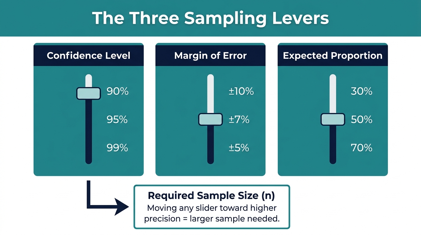
Before you touch any calculator, you need to understand the three levers you are pulling:
- Confidence level: How certain do you want to be that your results reflect the real population?
- Margin of error (confidence interval): How much "wiggle room" are you willing to accept around your estimate?
- Expected proportion: What share of the population do you expect to answer "yes" (or exhibit the behavior you are measuring)?
These three inputs drive everything. Let me walk through each one.
The Three Core Concepts, Explained Simply
Confidence Level
Confidence level is the probability that your sample result falls within your margin of error of the true population value [5]. The two most common choices are:
- 90% (used when resources are tight and stakes are moderate)
- 95% (the humanitarian and development sector standard)
- 99% (reserved for high-stakes research where being wrong has serious consequences)
A 95% confidence level means that if you ran your survey 100 times, 95 of those runs would produce a result within your margin of error. It does NOT mean you are 95% confident your specific result is correct, a subtle but important distinction.
💡 Tip: For most MEL field surveys (PDMs, needs assessments, KAP baselines), 95% confidence is the sweet spot. Going to 99% can nearly double your required sample size, often without a proportional benefit to decision-making.
Margin of Error
The margin of error tells you how much your sample estimate might differ from the true population value [2]. If you find that 60% of households are food insecure and your margin of error is ±5%, the true value is somewhere between 55% and 65%.
Smaller margins of error require larger samples. That trade-off is non-negotiable [4]. In practice, most humanitarian surveys accept a margin of error between ±5% and ±10%, depending on how the results will be used.
⚠️ Warning: A ±10% margin of error sounds manageable, but if you are measuring a low-prevalence indicator (say, 12% acute malnutrition), a ±10% swing makes your result nearly uninterpretable. For sensitive or low-prevalence indicators, tighten your margin.
Expected Proportion
Most sampling formulas ask for an "expected proportion", your best guess at what percentage of the population has the characteristic you are measuring. If you genuinely have no idea, use 50%, because this is the most conservative assumption and produces the largest (most protective) sample size [5].
The Australian Bureau of Statistics sample size guidance confirms this directly: to be 95% confident with a ±5% margin of error and an expected proportion of 50%, the required sample size is 385, a number you will see quoted across the sector [5].
The Magic Number 385 (and When to Trust It)
For large or unknown population sizes, you will often hear "just use 385." That number comes from the standard formula applied at 95% confidence, ±5% margin of error, and 50% expected proportion. It is a legitimate, defensible floor.
But here is what people often skip: 385 assumes a simple random sample from an infinite population. The moment you cluster your sampling (by village, by health facility, by distribution point), your effective precision drops. This is where the design effect comes in.
📝 Note: UNICEF's MICS sampling manual specifically flags that the design effect must be factored into your calculation when you are using cluster sampling, and it almost always inflates your required sample size [3]. A typical design effect of 1.5 to 2.0 means you may need 577 to 770 interviews to achieve the same precision as 385 simple random sample interviews.
The formula for adjusting is straightforward:
Adjusted sample size = Base sample size x Design effect
If you are doing a cluster survey in rural communities and assume a design effect of 1.5, your target jumps from 385 to about 578 completed interviews.
A Practical Decision Table for Field Contexts
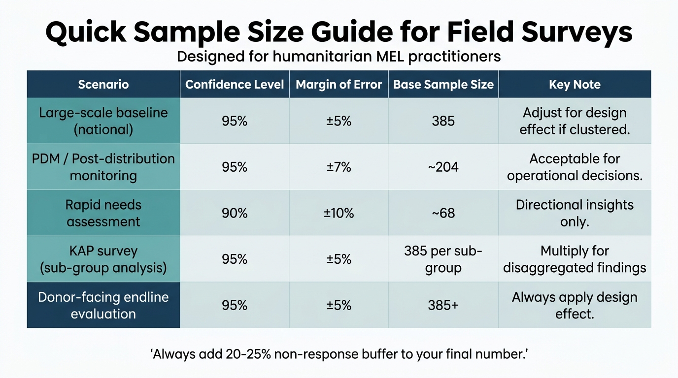
Here is the kind of quick-reference guide I use when helping teams scope surveys:
| Scenario | Confidence Level | Margin of Error | Base Sample (n) | Notes |
|---|---|---|---|---|
| Large-scale baseline (national) | 95% | ±5% | 385 | Adjust for design effect if clustered |
| PDM / post-distribution monitoring | 95% | ±7% | ~204 | Often acceptable for operational decisions |
| Rapid needs assessment | 90% | ±10% | ~68 | Use only for directional insights |
| KAP survey (sub-group analysis) | 95% | ±5% | 385 per sub-group | Multiply if you need disaggregated findings |
| Endline / evaluation (donor-facing) | 95% | ±5% | 385+ | Always apply design effect; consult ToR |
💡 Tip: If your survey results will be disaggregated by gender, geography, or vulnerability category, size your sample for each sub-group independently, not for the total population. This is one of the most common mistakes I see in field survey designs.
Two Sampling Goals People Confuse
Sawtooth Software's guide makes an important distinction that almost every other resource glosses over: there is a difference between sizing your sample for precision (confidence intervals and margin of error) and sizing it for power (hypothesis testing) [1].
Most MEL surveys are after precision: "What percentage of our beneficiaries have improved access to clean water?" That is a descriptive question, and the margin-of-error framework handles it well.
But if your evaluation is testing a hypothesis ("Did our intervention produce a statistically significant change compared to a control group?"), you need a power calculation, a different formula entirely, one that accounts for the size of the effect you expect to detect. This is where many mid-term and final evaluations underpower their designs without realizing it.
⚠️ Warning: If your evaluation TOR includes any language about "measuring impact" or "comparing treatment and control," ask your evaluator whether a power calculation was done. A sample sized for precision only may leave you unable to detect a real program effect.
Field Realities: Adjusting for Non-Response
No matter what your calculated sample size is, build in a non-response buffer. A standard adjustment is to divide your target sample by the expected response rate.
If you expect an 80% response rate (common in door-to-door household surveys) and your target is 385 completed interviews:
Households to approach = 385 / 0.80 = 482
Qualtrics and most survey methodology guides reinforce this point: attrition, refusals, and incomplete interviews are unavoidable, and your design should account for them upfront [4].
What I Actually Recommend for Most MEL Teams
If you are not a trained statistician and you are designing a field survey, here is my honest shorthand:
- Start with the Australian Bureau of Statistics or Qualtrics online calculators, they are free, reliable, and require no formula knowledge [4][5].
- Default to 95% confidence and ±5% margin of error unless your TOR or donor specifies otherwise.
- Use 50% as your expected proportion if you have no prior data.
- Apply a design effect if you are using cluster or stratified sampling, even a conservative 1.5 is better than ignoring it entirely [3].
- Add a 20-25% non-response buffer to your final number.
- Plan for sub-group sample sizes separately if disaggregated analysis is required.
If you want help turning these principles into a ready-to-use sampling plan or an actual survey instrument, that is exactly the kind of work I do. You can start at vera.ignex.io, no jargon, no statistics degree required.
The Bottom Line
Sample size is not about achieving statistical perfection. It is about making a transparent, documented decision that balances rigor with field reality. The goal is a sample that is defensible to your donor, meaningful to your program team, and achievable by your data collectors.
You do not need to become a statistician to get this right. You just need to understand the three levers, know when to apply a design effect correction, and be honest about your trade-offs. That is something every MEL practitioner can do.
Sources
- Figuring Out Sample Size for Survey Research — Sawtooth Software
- How to Determine Sample Size for a Research Study — GeoPoll
- MICS4 Manual: Designing and Selecting the Sample — UNICEF
- Sample Size Calculator and Margin of Error: The Ultimate Guide — Appinio
- Sample Size Calculator Help — Australian Bureau of Statistics
- Sample Size Calculator — Qualtrics
Put this into practice with Vera
Build logframes, indicators, surveys and reports in minutes — with an AI made for MEL.
Try Vera free →